Protect a sdc_raster by smoothing

protect_smooth reduces the sensitivity by applying a Gaussian smoother, making the values less localized.

Usage

protect_smooth(x, bw = raster::res(x$value), ...)

Arguments

x

raster object

bw

bandwidth

...

passed through to focal.

Details

The sensitivity of a raster can be decreased by applying a kernel density smoother as argued by de Jonge et al. (2016) and de Wolf et al. (2018). Smoothing spatially spreads localized values, reducing the risk for location disclosure. Note that smoothing often visually enhances detection of spatial patterns. The kernel applied is a Gaussian kernel with a bandwidth bw supplied by the user. The smoother acts upon the x$value$count and x$value$sum from which a new x$value$mean is derived.

References

de Jonge, E., & de Wolf, P. P. (2016, September). Spatial smoothing and statistical disclosure control. In International Conference on Privacy in Statistical Databases (pp. 107-117). Springer, Cham.

de Wolf, P. P., & de Jonge, E. (2018, September). Safely Plotting Continuous Variables on a Map. In International Conference on Privacy in Statistical Databases (pp. 347-359). Springer, Cham.

See also

Other protection methods: protect_quadtree(), remove_sensitive()

Examples

# \donttest{
library(sdcSpatial)
library(raster)

data(enterprises)

# create a sdc_raster from point data with raster with
# a resolution of 200m
production <- sdc_raster(enterprises, variable = "production"
                        , r = 200, min_count = 3)

print(production)
#> numeric sdc_raster object: 
#>    resolution: 200 200 ,  max_risk: 0.95 , min_count: 3 
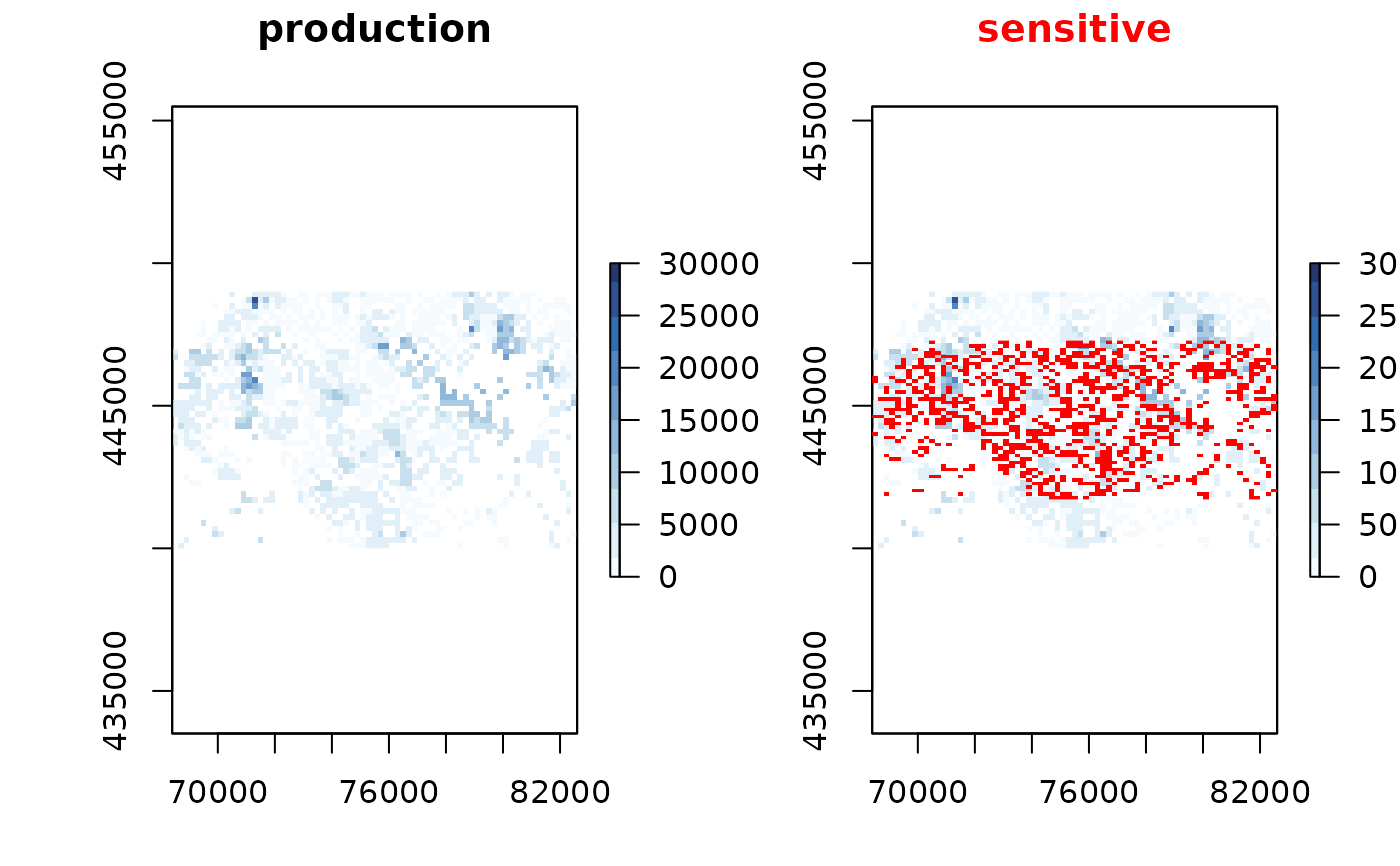
#>    mean sensitivity score [0,1]:  0.6328234

# plot the raster
zlim <- c(0, 3e4)
# show which raster cells are sensitive
plot(production, zlim=zlim)


# but we can also retrieve directly the raster
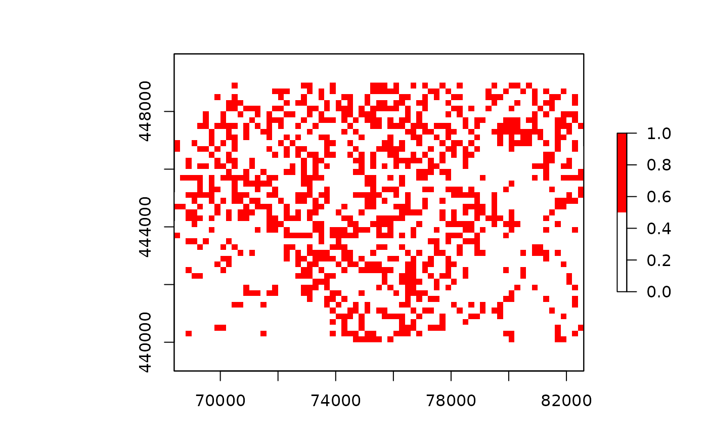
sensitive <- is_sensitive(production, min_count = 3)
plot(sensitive, col = c('white', 'red'))


# what is the sensitivy fraction?
sensitivity_score(production)
#> [1] 0.6328234
# or equally
cellStats(sensitive, mean)
#> [1] 0.6328234

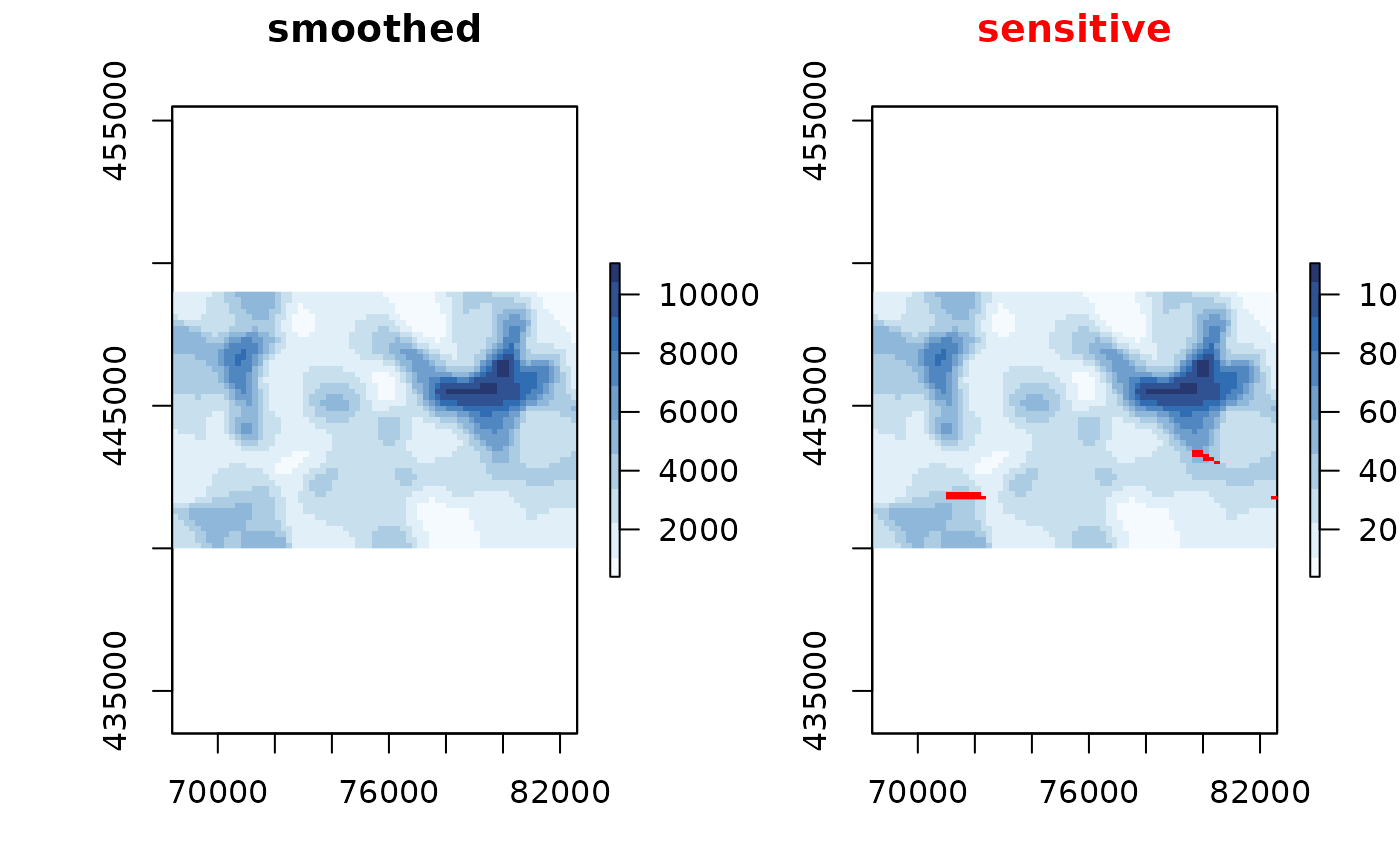
# let's smooth to reduce the sensitivity
smoothed <- protect_smooth(production, bw = 400)
plot(smoothed)


# let's smooth to reduce the sensitivity, with higher resolution
smoothed <- protect_smooth(production, bw = 400, smooth_fact=4, keep_resolution=FALSE)
plot(smoothed)


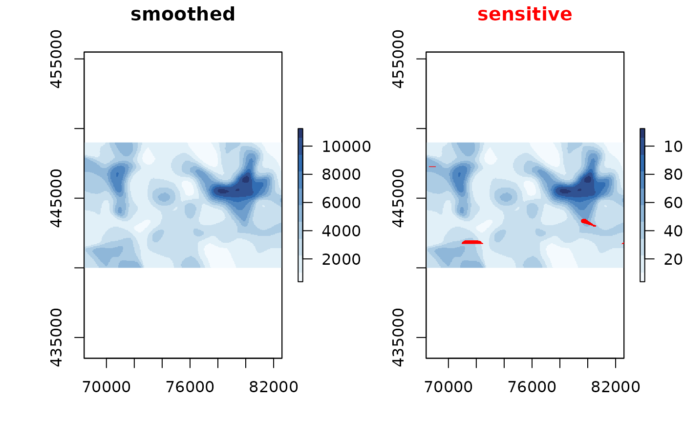# what is the sensitivy fraction?
sensitivity_score(smoothed)
#> [1] 0.007902973

# let's remove the sensitive data.
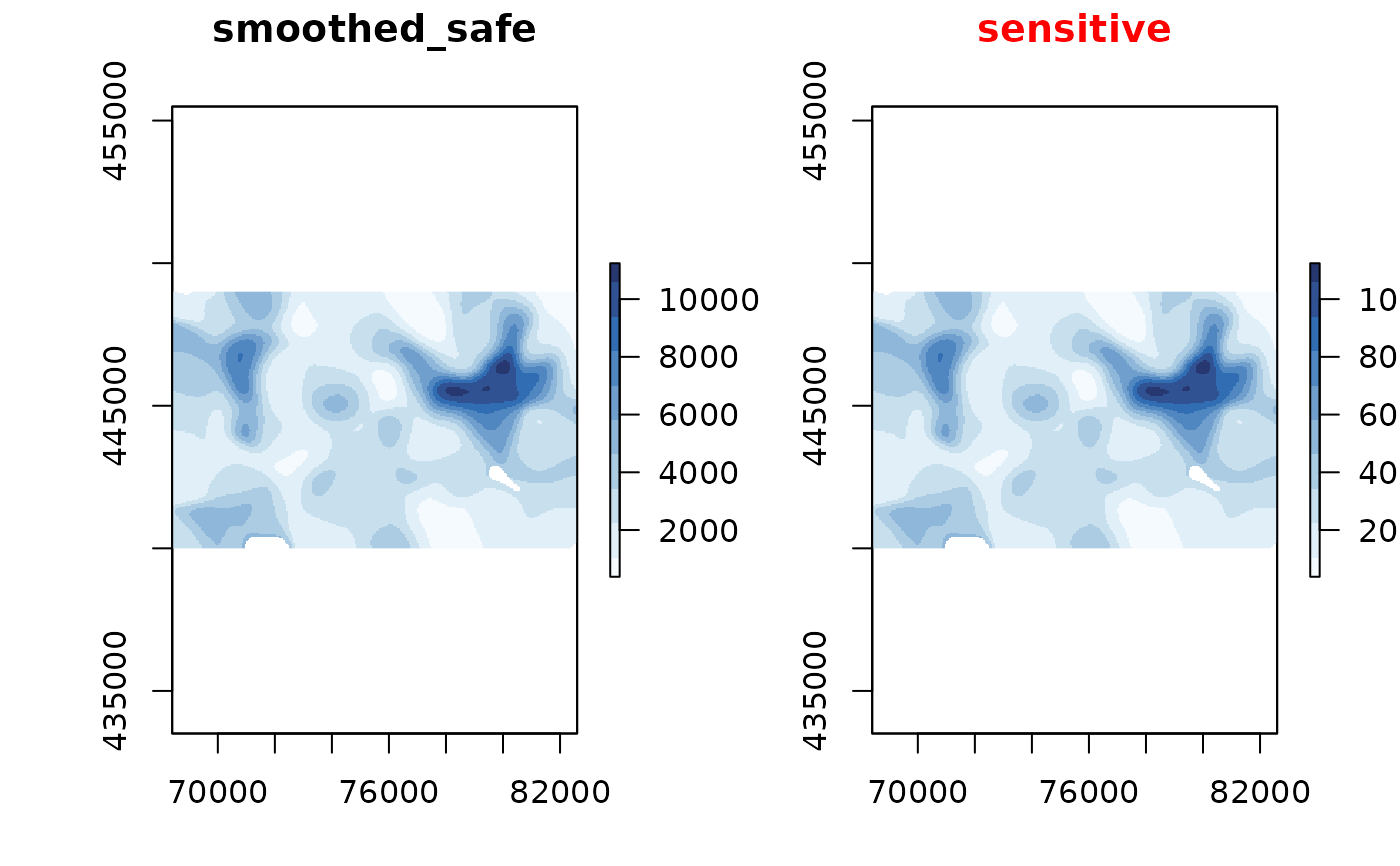
smoothed_safe <- remove_sensitive(smoothed, min_count = 3)
plot(smoothed_safe)


# let's communicate!
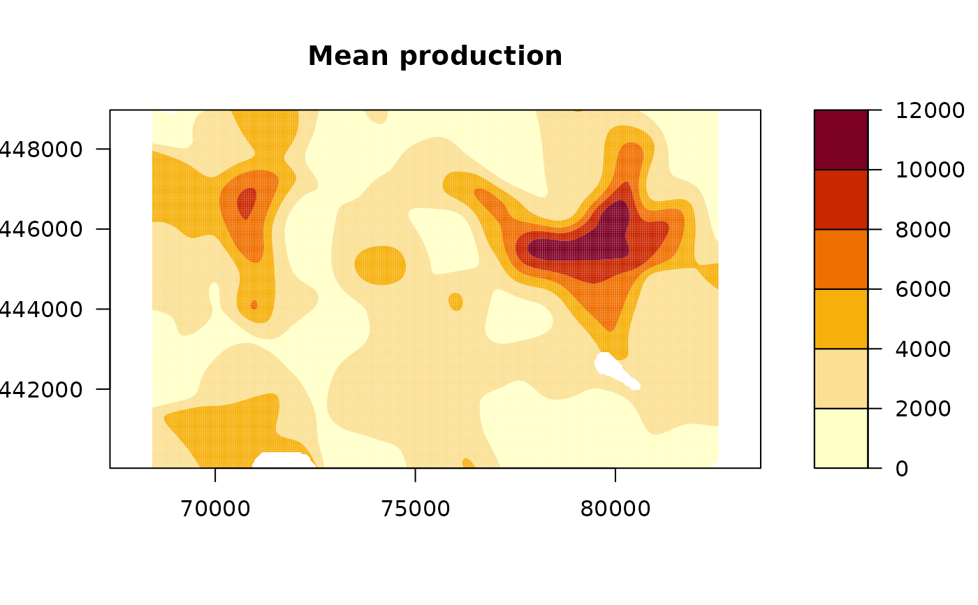
production_mean <- mean(smoothed_safe)
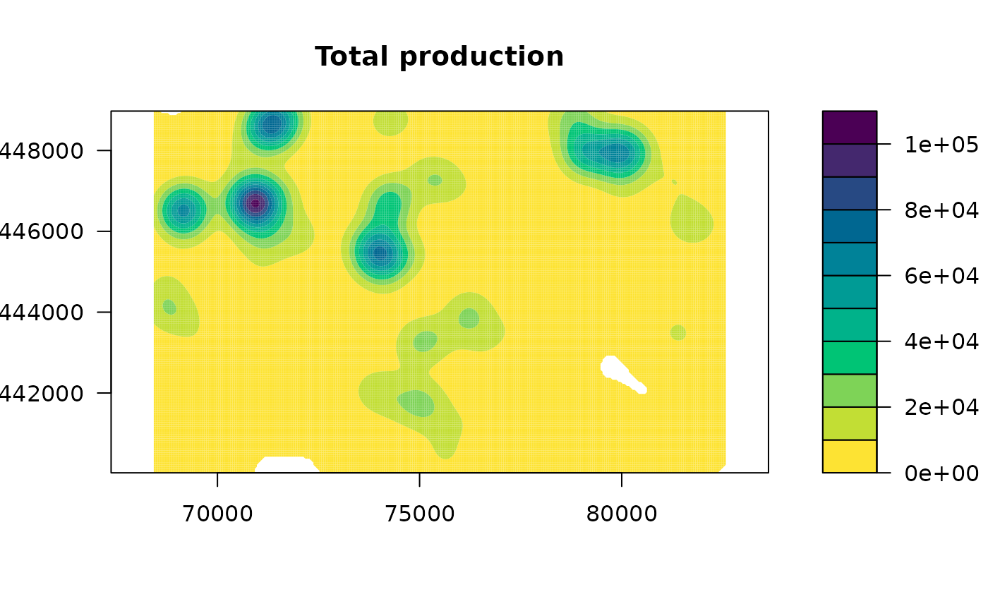
production_total <- sum(smoothed_safe)

# and create a contour plot
raster::filledContour(production_mean, nlevels = 6, main = "Mean production")



# generated with R 3.6 >=
#col <- hcl.colors(11, rev=TRUE)
col <- c("#FDE333", "#C2DE34", "#7ED357", "#00C475", "#00B28A", "#009B95"
        ,  "#008298", "#006791", "#274983", "#44286E", "#4B0055"
        )
raster::filledContour(production_total, nlevels = 11
             , col = col
             , main="Total production")

# }