The data are generated with residence/household locations from the Dutch open data BAG register. The locations are realistic, but the associated data is simulated.
Format
a data.frame with 90603 rows and 4 columns.
- x
integer, x coordinate of dwelling (crs 28992)
- y
integer, y coordinate of dwelling (crs 28992)
- consumption
numeric, simulated continuous value
- unemployed
logical, simulated discrete value
Source
Basisregistratie Adressen en Gebouwen https://www.kadaster.nl/zakelijk/registraties/basisregistraties/bag/bag-producten
Examples
# \donttest{
# dwellings is a data.frame, the best way is to first turn it
# into a sf or sp object.
# create an sf object from our data
if (requireNamespace("sf")){
dwellings_sf <- sf::st_as_sf(dwellings, coords=c("x", "y"), crs=28992)
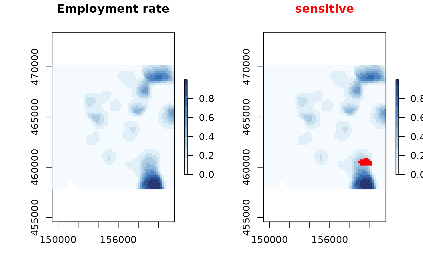
unemployed <- sdc_raster( dwellings_sf
, "unemployed"
, r=200
, max_risk = 0.9
)
plot(unemployed)
sensitivity_score(unemployed)
unemployed_smoothed <- protect_smooth(unemployed, bw = 0.4e3)
plot(unemployed_smoothed, main="Employment rate")
plot(unemployed_smoothed, "sum", main = "Employment")
} else {
message("Package 'sf' was not installed.")
}
#> Loading required namespace: sf

 dwellings_sp <- dwellings
# or change a data.frame into a sp object
sp::coordinates(dwellings_sp) <- ~ x + y
tryCatch(
# not working on some OS versions.
sp::proj4string(dwellings_sp) <- "+init=epsg:28992"
)
#> Warning: GDAL Message 1: +init=epsg:XXXX syntax is deprecated. It might return a CRS with a non-EPSG compliant axis order.
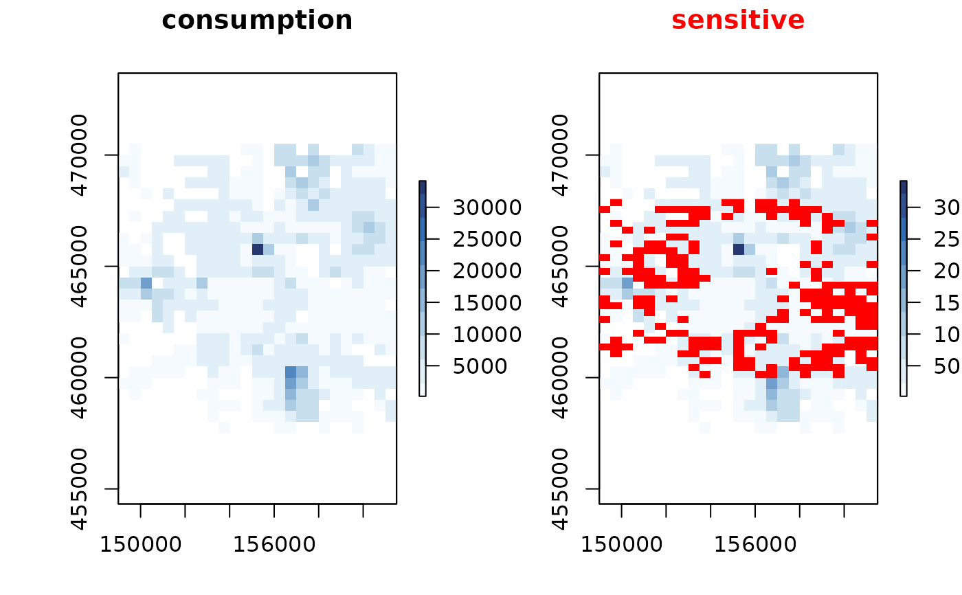
consumption <- sdc_raster(dwellings_sp, dwellings_sp$consumption, r = 500)
consumption
#> numeric sdc_raster object:
#> resolution: 500 500 , max_risk: 0.95 , min_count: 10
#> mean sensitivity score [0,1]: 0.4207188
plot(consumption)
dwellings_sp <- dwellings
# or change a data.frame into a sp object
sp::coordinates(dwellings_sp) <- ~ x + y
tryCatch(
# not working on some OS versions.
sp::proj4string(dwellings_sp) <- "+init=epsg:28992"
)
#> Warning: GDAL Message 1: +init=epsg:XXXX syntax is deprecated. It might return a CRS with a non-EPSG compliant axis order.
consumption <- sdc_raster(dwellings_sp, dwellings_sp$consumption, r = 500)
consumption
#> numeric sdc_raster object:
#> resolution: 500 500 , max_risk: 0.95 , min_count: 10
#> mean sensitivity score [0,1]: 0.4207188
plot(consumption)
 # but we can also create a raster directly from a data.frame
unemployed <- sdc_raster( dwellings[c("x","y")], dwellings$unemployed)
# }
# but we can also create a raster directly from a data.frame
unemployed <- sdc_raster( dwellings[c("x","y")], dwellings$unemployed)
# }